Implementing Linear Regression using Stats Models

Introduction to Linear Regression

Linear Regression or Ordinary Least Squares Regression (OLS) is one of the simplest machine learning algorithms and produces both accurate and interpretable results on most types of continuous data. While more sophisticated algorithms like random forest will produce more accurate results, they are know as “black box” models because it’s tough for analysts to interpret the model. In contrast, OLS regression results are clearly interpretable because each predictor value (beta) is assigned a numeric value (coefficient) and a measure of significance for that variable (p-value). This allows the analyst to interpret the effect of difference predictors on the model and tune it easily.

Here we’ll use college admissions data and the statsmodels package to perform a simple linear regression looking at the relationship between average SAT score, out-of-state tuition and the selectivity for a range of US higher education institutions. We'll read the data using pandas and represent it visually using matplotlib.

import pandas as pd
import statsmodels.api as sm
import matplotlib.pyplot as plt
%matplotlib inline

cols = ['ADM_RATE','SAT_AVG', 'TUITIONFEE_OUT'] #cols to read, admit rate, avg sat score & out-of-state tuition

df = pd.read_csv('college_stats.csv', usecols=cols)
df.dropna(how='any', inplace=True)
len(df) #1303 schools

Represent the OLS Results Numerically

#fit X & y
y,X=(df['TUITIONFEE_OUT'], df[['SAT_AVG','ADM_RATE']])

#call the model
model = sm.OLS(y, X)

#fit the model
results = model.fit()

#view results
results.summary()

OLS Regression Results
Dep. Variable:	TUITIONFEE_OUT	R-squared:	0.919
Model:	OLS	Adj. R-squared:	0.919
Method:	Least Squares	F-statistic:	7355.
Date:	Sat, 24 Jun 2017	Prob (F-statistic):	0.00
Time:	12:11:48	Log-Likelihood:	-13506.
No. Observations:	1303	AIC:	2.702e+04
Df Residuals:	1301	BIC:	2.703e+04
Df Model:	2
Covariance Type:	nonrobust

	coef	std err	t	P>\|t\|	[95.0% Conf. Int.]
SAT_AVG	29.8260	0.577	51.699	0.000	28.694 30.958
ADM_RATE	-9600.6540	907.039	-10.585	0.000	-1.14e+04 -7821.235

Omnibus:	9.845	Durbin-Watson:	1.313
Prob(Omnibus):	0.007	Jarque-Bera (JB):	7.664
Skew:	-0.090	Prob(JB):	0.0217
Kurtosis:	2.670	Cond. No.	4.55e+03

Note that although we only used two variables we get a strong R-squared. This means that much of the variability within the out-of-state tuition can be explained or captured by SAT scores and selectivity or admittance rate.

Represent the OLS Results Visually

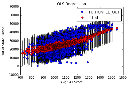
Plot of Out of State Tuition and Average SAT Score

fig, ax = plt.subplots()
fig = sm.graphics.plot_fit(results, 0, ax=ax)
ax.set_ylabel("Out of State Tuition")
ax.set_xlabel("Avg SAT Score")
ax.set_title("OLS Regression")

<matplotlib.text.Text at 0x10b6cd790>

png

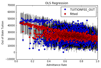
Plot of Out of State Tuition and Admittance Rate

fig, ax = plt.subplots()
fig = sm.graphics.plot_fit(results, 1, ax=ax)
ax.set_ylabel("Out of State Tuition")
ax.set_xlabel("Admittance Rate")
ax.set_title("OLS Regression")

<matplotlib.text.Text at 0x10cfd4390>

png