Classifying Charity Donors
Classifying Charity Donors
In this project, I will employed several supervised algorithms to accurately model individuals' income using data collected from the 1994 U.S. Census. I then identified the best candidate algorithm from preliminary results and further optimized this algorithm to best model the data.
The goal of this analysis is to construct a model that accurately predicts whether an individual makes more than $50,000 USD annually. This sort of task can is common in a non-profit settings, where organizations survive on donations.
Armed with information on an individual's income level aids non-profits in understanding how large of a donation to request, or whether they should contact certain individuals begin with. While it can be difficult to determine an individual's general income, we can (as we will see) infer this value from other publicly available features such as government census studies.
The dataset for this project originates from the UCI Machine Learning Repository. The datset was donated by Ron Kohavi and Barry Becker, after being published in the article "Scaling Up the Accuracy of Naive-Bayes Classifiers: A Decision-Tree Hybrid". You can find the article by Ron Kohavi online. The data we investigate here consists of small changes to the original dataset, such as removing the 'fnlwgt' feature and records with missing or ill-formatted entries.
I completed this project as part of the Udacity Machine Learning Engineer Nano Degree
# Import libraries necessary for this project
import numpy as np
import pandas as pd
from time import time
from IPython.display import display # Allows the use of display() for DataFrames
from __future__ import division #for division


# Import supplementary visualization code
import visuals as vs

# Pretty display for notebooks
%matplotlib inline

# Load the Census dataset
data = pd.read_csv("census.csv")

# Success - Display the first record
display(data.head(1))
| age | workclass | education_level | education-num | marital-status | occupation | relationship | race | sex | capital-gain | capital-loss | hours-per-week | native-country | income | |
|---|---|---|---|---|---|---|---|---|---|---|---|---|---|---|
| 0 | 39 | State-gov | Bachelors | 13 | Never-married | Adm-clerical | Not-in-family | White | Male | 2174 | 0 | 40 | United-States | <=50K |
#summary stats
data.describe().astype(int)
| age | education-num | capital-gain | capital-loss | hours-per-week | |
|---|---|---|---|---|---|
| count | 45222 | 45222 | 45222 | 45222 | 45222 |
| mean | 38 | 10 | 1101 | 88 | 40 |
| std | 13 | 2 | 7506 | 404 | 12 |
| min | 17 | 1 | 0 | 0 | 1 |
| 25% | 28 | 9 | 0 | 0 | 40 |
| 50% | 37 | 10 | 0 | 0 | 40 |
| 75% | 47 | 13 | 0 | 0 | 45 |
| max | 90 | 16 | 99999 | 4356 | 99 |
Data Exploration
As a preliminary step let's determine how many individuals within our data set fall into each of our two buckets: - Individuals making more than \$50K annually - Individuals making less than \$50K annually
Also bear in mind that this census data was from 1994 and annual wages have inflated since then.
# Total number of records
n_records = data.shape[0]

# Number of records where individual's income is more than $50,000
n_greater_50k = data.income.value_counts()[1].astype(int)

# Number of records where individual's income is at most $50,000
n_at_most_50k = data.income.value_counts()[0].astype(int)

# Percentage of individuals whose income is more than $50,000
greater_percent = n_greater_50k / n_records

# Print the results
print "Total number of records: {}".format(n_records)
print "Individuals making more than $50,000: {}".format(n_greater_50k)
print "Individuals making at most $50,000: {}".format(n_at_most_50k)
print "Percentage of individuals making more than $50,000: {:.2f}%".format(greater_percent * 100)
Total number of records: 45222
Individuals making more than $50,000: 11208
Individuals making at most $50,000: 34014
Percentage of individuals making more than $50,000: 24.78%
Data Pre-Processing
Before we move on to modeling we're going to perform some preprocessing on our dataset to adjust the quality of our variables. For example, since we’re dealing with a monetary response variable income, it’s common to perform log transformations to normalize its distribution.
# Split the data into features and target label
income_raw = data['income']
features_raw = data.drop('income', axis = 1)
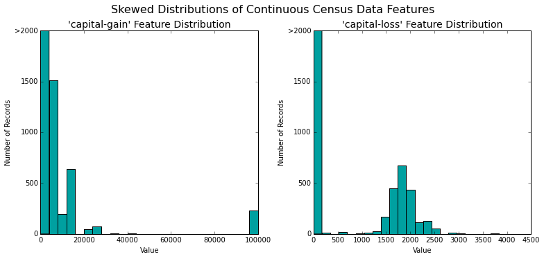
# Visualize skewed continuous features of original data
vs.distribution(data)
Log Transformation
Notice the strong positive skew present in the capital-gain and capital-loss features. In order to compress the range of our dataset and deal with outliers we will perform a log transformation using np.log(). However, it's important to remember that the log of zero is undefined so we will add 1 to each sample.
# Log-transform the skewed features
skewed = ['capital-gain', 'capital-loss']
features_raw[skewed] = data[skewed].apply(lambda x: np.log(x + 1)) #add 1

# Visualize the new log distributions
vs.distribution(features_raw, transformed = True)
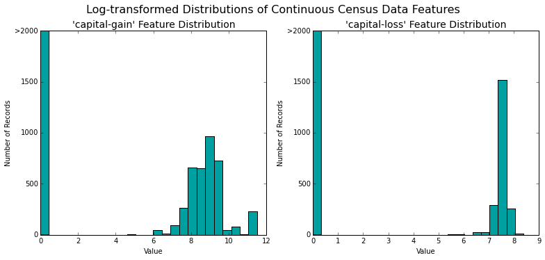
The new distribution, which is still non-normally distributed, is much better than our initial state. This effect is more pronounced on the capital-gain feature.
Scaling (Normalizing) Numeric Features
After implementing our log transformation, it's good practice to perform scaling on numerical features so that each feature will be weighted equally when we have our algorithm ingest it. NOTE: once scaling has been applied, the features will not be recognizable.
To do this we'll employ sklearn's sklearn.preprocessing.MinMaxScaler. Any outliers will dramatically effect the results of the scaling, that's why we handled them with a log transformation in the previous step. What's happening under-the-hood of this function is a simple division and subtraction to re-weight each sample within each feature such that they all fall within the range (0,1). The math behind the function is displayed below:
%%latex

$$\ x_{scaled}=\frac{X - X_{min}}{X_{max} - X_{min}} $$
$$\ x_{scaled}=\frac{X - X_{min}}{X_{max} - X_{min}} $$
from sklearn.preprocessing import MinMaxScaler

# Initialize a scaler, then apply it to the features
scaler = MinMaxScaler()
numerical = ['age', 'education-num', 'capital-gain', 'capital-loss', 'hours-per-week']
features_raw[numerical] = scaler.fit_transform(data[numerical])

# Show an example of a record with scaling applied
display(features_raw.head(1))
| age | workclass | education_level | education-num | marital-status | occupation | relationship | race | sex | capital-gain | capital-loss | hours-per-week | native-country | |
|---|---|---|---|---|---|---|---|---|---|---|---|---|---|
| 0 | 0.30137 | State-gov | Bachelors | 0.8 | Never-married | Adm-clerical | Not-in-family | White | Male | 0.02174 | 0 | 0.397959 | United-States |
Encoding Categorical Features
Now that the numeric features have been transformed and scaled, it's time to give our categorical features some love. Since most machine learning algorithms will expect all features to be numeric, we'll perform feature encoding using pandas pd.get_dummies() function which will transform category values into numeric dummy variables within a dataframe.
We'll also encode the the response variable (income) with 0 = income less than \$50K and 1 = income greater than \$50K.
# Encode categorical features
features = pd.get_dummies(features_raw)

# Encode the 'income_raw' data to numerical values
income = income_raw.replace({ '<=50K' : 0, '>50K' : 1})

# Print the number of features after one-hot encoding
encoded = list(features.columns)
print "{} total features after encoding.".format(len(encoded))
103 total features after encoding.
Shuffle Split the Data
Now that we've transformed and scaled our numeric features and encoded both our categorical features as well as our response variable we're ready to split our data set into training and testing sets.
# Import train_test_split
from sklearn.cross_validation import train_test_split

# Split the 'features' and 'income' data into training and testing sets
X_train, X_test, y_train, y_test = train_test_split(features, income, test_size = 0.2, random_state = 0)

# Show the results of the split
print "Training set has {} samples.".format(X_train.shape[0])
print "Testing set has {} samples.".format(X_test.shape[0])
Training set has 36177 samples.
Testing set has 9045 samples.
Establishing a Baseline Model
If we create a mode always predicted an individual made more than \$50,000, what would that model's accuracy and F-score be on this dataset?
Let's test this out to serve as a baseline to compare our other learning algorithms's performance.
from sklearn.metrics import confusion_matrix
from sklearn.metrics import accuracy_score

#naive classifier
y_pred = income.replace(0,1)

#confusion matrix
cm = confusion_matrix(income,y_pred)

#metrics
tn = cm[0,0]
fp = cm[0,1]
fn = cm[1,0]
tp = cm[1,1]

recall = tp / (tp + fn)
precision = tp / (tp + fp)

beta = .5

# Calculate accuracy
accuracy = (tp + tn) / (tp + tn + fp + fn)

# Calculate F-score using the formula above for beta = 0.5

fscore = (1 + beta**2) * ((precision * recall) / ((beta**2 * precision) + recall))

# Print the results
print "Naive Predictor: [Accuracy score: {:.4f}, F-score: {:.4f}]".format(accuracy, fscore)
Naive Predictor: [Accuracy score: 0.2478, F-score: 0.2917]
As expected, the Naive Predictor's accuracy is equal to the number of individuals making over \$50K. Let's see if we can create a model which does a better job at predicting!
Classification & Training — Creating a Modeling Pipeline
from sklearn.metrics import accuracy_score, fbeta_score #metrics / scoring
from sklearn.naive_bayes import GaussianNB
from time import time

def train_predict(learner, sample_size, X_train, y_train, X_test, y_test):
    '''
    inputs:
       - learner: the learning algorithm to be trained and predicted on
       - sample_size: the size of samples (number) to be drawn from training set
       - X_train: features training set
       - y_train: income training set
       - X_test: features testing set
       - y_test: income testing set
    '''

    results = {}

    # Fit the learner to the training data using slicing with 'sample_size'
    start = time() # Get start time
    learner = learner.fit(X_train[:sample_size], y_train[:sample_size]) #sample_weight=sample_size
    end = time() # Get end time

    # Calculate the training time
    results['train_time'] = (end - start)

    # Get the predictions on the test set,
    #       then get predictions on the first 300 training samples
    start = time() # Get start time
    predictions_test = learner.predict(X_test) #pred = clf.predict(features_test)
    predictions_train = learner.predict(X_train[:300])
    end = time() # Get end time

    # Total prediction time
    results['pred_time'] = (end - start)

    # Compute accuracy on 300 training samples
    results['acc_train'] = accuracy_score(y_train[:300], predictions_train)

    # Compute accuracy on test set
    results['acc_test']  = accuracy_score(y_test, predictions_test)


    # Compute F-score on 300 training samples
    results['f_train'] = fbeta_score(y_train[:300], predictions_train, beta=.5)


    # Compute F-score on the test set
    results['f_test'] = fbeta_score(y_test, predictions_test, beta=.5)

    # Success
    print "{} trained on {} samples.".format(learner.__class__.__name__, sample_size)

    # Return the results
    return results

train_predict(GaussianNB(), 36177, X_train, y_train,X_test, y_test)
GaussianNB trained on 36177 samples.


{'acc_test': 0.60829187396351581,
 'acc_train': 0.59333333333333338,
 'f_test': 0.42811288507232487,
 'f_train': 0.41249999999999998,
 'pred_time': 0.028007984161376953,
 'train_time': 0.12101292610168457}
Selecting Algorithm Candidates
| Application Example | Strengths | Weaknesses | Why this is a good model for this specific problem |
|---|---|---|---|
| Gaussian Naive Bayes (GaussianNB) - "Naive Bayes spam filtering is a baseline technique for dealing with spam that can tailor itself to the email needs of individual users and give low false positive spam detection rates that are generally acceptable to users. It is one of the oldest ways of doing spam filtering, with roots in the 1990s." Source |
|
|
Since we're trying to bucket individuals into income brackets NB's algorithm is a good candidate. If we were trying to predict an individual's exact income I would be less inclined to use this algorithm. |
| Logistic Regression - "Logistic regression is used in various fields, including machine learning, most medical fields, and social sciences." It lends itself particularly well to binary classification tasks common in medical research, such as classifying whether someone has a certain illness or not."For example, the Trauma and Injury Severity Score (TRISS), which is widely used to predict mortality in injured patients, was originally developed by Boyd et al. using logistic regression." Source |
|
|
Logistic Regression is one of the most basic flavors of classification algorithms and since that's exactly the task at hand it appears to be a good candidate to test. |
| Random Forest - "Or random decision forests[1][2] are an ensemble learning method for classification, that operates by constructing a multitude of decision trees at training time and outputting the class that is the mode of the classes (classification) or mean prediction (regression) of the individual trees. Random decision forests correct for decision trees' habit of overfitting to their training set." Random Forests are one of the most flexible and elegant ML algorithms and they have been applied to a wide range of fields including predicting the quality of surveys using NLP Source |
|
|
Random Forests algorithm is the bread and butter for many machine learning tasks due to its flexibility and ability to correct individual decision trees proneness to overfitting by sampling many of them. I hypothesize this algorithm will out perform the other two. |
Model Comparison / Evaluation
Great now that we've estabilished a modeling pipeline, established baseline performance and selecte two other algorithms we can now, finally, get to modeling.
# Import the three supervised learning models from sklearn
from sklearn.naive_bayes import GaussianNB
from sklearn.linear_model import LogisticRegression
from sklearn.ensemble import RandomForestClassifier, ExtraTreesClassifier

#2 creating classifier
# Initialize the three models
clf_A = GaussianNB()
clf_B = LogisticRegression(random_state = 0)
clf_C = RandomForestClassifier(random_state = 0)


# Calculate the number of samples for 1%, 10%, and 100% of the training data
samples_1 = X_train.shape[0]*0.01; samples_1 = int(samples_1)
samples_10 = X_train.shape[0]*0.1; samples_10 = int(samples_10)
samples_100 = X_train.shape[0]; samples_100 = int(samples_100)

# Collect results on the learners
results = {}
for clf in [clf_A, clf_B, clf_C]:
    clf_name = clf.__class__.__name__
    results[clf_name] = {}
    for i, samples in enumerate([samples_1, samples_10, samples_100]):
        results[clf_name][i] = \
        train_predict(clf, samples, X_train, y_train, X_test, y_test)

# Run metrics visualization for the three supervised learning models chosen
vs.evaluate(results, accuracy, fscore)
GaussianNB trained on 361 samples.
GaussianNB trained on 3617 samples.
GaussianNB trained on 36177 samples.
LogisticRegression trained on 361 samples.
LogisticRegression trained on 3617 samples.
LogisticRegression trained on 36177 samples.
RandomForestClassifier trained on 361 samples.
RandomForestClassifier trained on 3617 samples.
RandomForestClassifier trained on 36177 samples.
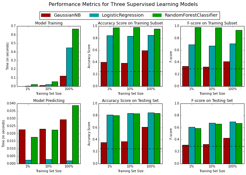
Model Selection
If we care most about the accuracy and speed of our classifier then based on our analysis of the three learning algorithms tested, I recommend we move forward with Logistic Regression because it outperforms both Naive Bayes and Random Forest in terms of prediction accuracy on our testing set and is much faster to train than random forest. Furthermore, it's F-score falls between the other two algorithms meaning we'd expect it to fall in the middle of our other two candidates on precision and recall.
LOGISTIC REGRESSION
- What's happening under-the-hood of logit regression?
We can think of a logit regression as being similar to a linear regression but with a discrete as opposed to continuous output. The classification algorithm draws an S-shaped decision boundary which, in our case, divides the two classes. For each sample within our dataset, the algorithm assigns a probability to determine which class the point would fall into. For example if we have two classes (0 = less than $50K & 1 = more than $50K), then (without any tuning of the decision boundary) points with a probability of less than .5 would be classified as 0 and points with greater than .5 probability would be classified as 1.
TL;DR: In this scenario Logistic Regression provides a model that is more accurate, easy to interpret and quicker to predict on our testing data.
Summary So Far
We rigorously tested three machine learning algorithms to determine which would predict a person's level of income and after our analysis we feel confident in moving forward with logistic regression because it provides high accuracy, ease of interpretability (we get coefficients for each predictor) and is able to quickly provide predictions.
In order to get this far we split our data into training and testing sets. But prior to this we normalized our targets by performing a log transformation on numeric target data, min-max scaling on all numeric predictor variables and one-hot-encoding on all categorical predictor features.
We then trained our models using different cuts of training data (1%, 10% and 100% of the sets) and at each cut logistic regression provided the most accurate results. After the model was trained we used our testing test to determine accuracy and F-scores of each model on data it had not been previously trained on. At this step Logistic regression fell in the middle of the other two algorithms in terms of precision and recall, meaning it had the most neutral bias-variance trade-off.
Model Tuning
Not that we've selected Logistic Regression as our model of choice, we can use sklearn's GridSearchCV function to tune our model using different permutations of parameters to our model
# Import 'GridSearchCV', 'make_scorer', and any other necessary libraries
from sklearn.metrics import accuracy_score, fbeta_score, make_scorer
from sklearn.linear_model import LogisticRegression, LogisticRegressionCV
from sklearn.grid_search import GridSearchCV

# Initialize the classifier

clf = LogisticRegression()

# Create the parameters list you wish to tune
parameters = [{'C': [0.01, 0.1, 1, 10],"solver" : ['newton-cg','liblinear']}]

# Make an fbeta_score scoring object
scorer = make_scorer(fbeta_score, beta=.5)


# Perform grid search on the classifier using 'scorer' as the scoring method
grid_obj =  GridSearchCV(LogisticRegression(penalty='l2', random_state=0),parameters ,scoring=scorer)


# Fit the grid search object to the training data and find the optimal parameters
grid_fit = grid_obj.fit(X_train, y_train)


# Get the estimator
best_clf = grid_fit.best_estimator_

# Make predictions using the unoptimized and model
predictions = (clf.fit(X_train, y_train)).predict(X_test)
best_predictions = best_clf.predict(X_test)

# Report the before-and-afterscores
print "Unoptimized model\n------"
print "Accuracy score on testing data: {:.4f}".format(accuracy_score(y_test, predictions))
print "F-score on testing data: {:.4f}".format(fbeta_score(y_test, predictions, beta = 0.5))
print "\nOptimized Model\n------"
print "Final accuracy score on the testing data: {:.4f}".format(accuracy_score(y_test, best_predictions))
print "Final F-score on the testing data: {:.4f}".format(fbeta_score(y_test, best_predictions, beta = 0.5))
Unoptimized model
------
Accuracy score on testing data: 0.8483
F-score on testing data: 0.6993

Optimized Model
------
Final accuracy score on the testing data: 0.8498
Final F-score on the testing data: 0.7018
Final Model Evaluation
Logistic Regression Optimized Results vs Naive Predictor's Baseline Results:
| Metric | Benchmark Predictor | Unoptimized Model | Optimized Model |
|---|---|---|---|
| Accuracy Score | 24.38% | 84.83% | 84.94% |
| F-score | .2442 | .6993 | .7008 |
As we can see from the comparison table above, our logistic model does a much better job at accurately predicting an individual's income and has a higher F-Score which means it does a better job of balancing precision and recall.
Extracting Feature Importance
Here we'll choose a different scikit-learn supervised learning algorithm that has a feature_importance_ attribute. This attribute is a function that ranks the importance of each feature when making predictions based on the chosen algorithm so we can gain an understanding of the underlying importance for each feature within our model.
# Import a supervised learning model that has 'feature_importances_'
from sklearn.ensemble import AdaBoostClassifier

# Train the supervised model on the training set
model = AdaBoostClassifier(n_estimators=100).fit(X_train, y_train)

# Extract the feature importances
importances = model.feature_importances_

# Plot
vs.feature_plot(importances, X_train, y_train)
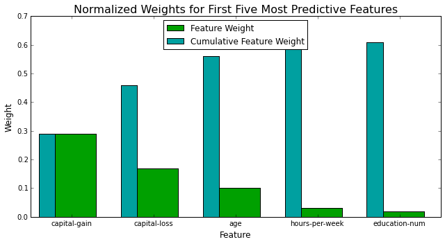
Interestingly capital-gain/loss, age, hours-per-week and education explain the most variane within the dataset.
Also interesting to note that the fives features here together account for ~60% of the total weight given to all predictors.
Feature Selection
How does the model perform if we only use a subset of all the available features in the data? With less features required to train, the time requird for training and prediction time is much lower — at the cost of performance metrics.
From the viz above, we see that the top five most important features explain about ~60% of the variance within the dataset. This means that we can potentially compress our feature space and simplify the information required for the model to learn. This code will compare our optimized model with a full feature set to a new optimized model using only the top 5 features.
# Import functionality for cloning a model
from sklearn.base import clone

# Reduce the feature space
X_train_reduced = X_train[X_train.columns.values[(np.argsort(importances)[::-1])[:5]]]
X_test_reduced = X_test[X_test.columns.values[(np.argsort(importances)[::-1])[:5]]]

# Train on the "best" model found from grid search earlier
clf = (clone(best_clf)).fit(X_train_reduced, y_train)

# Make new predictions
reduced_predictions = clf.predict(X_test_reduced)

# Report scores from the final model using both versions of data
print "Final Model trained on full data\n------"
print "Accuracy on testing data: {:.4f}".format(accuracy_score(y_test, best_predictions))
print "F-score on testing data: {:.4f}".format(fbeta_score(y_test, best_predictions, beta = 0.5))
print "\nFinal Model trained on reduced data\n------"
print "Accuracy on testing data: {:.4f}".format(accuracy_score(y_test, reduced_predictions))
print "F-score on testing data: {:.4f}".format(fbeta_score(y_test, reduced_predictions, beta =.5))
Final Model trained on full data
------
Accuracy on testing data: 0.8498
F-score on testing data: 0.7018

Final Model trained on reduced data
------
Accuracy on testing data: 0.8092
F-score on testing data: 0.5998
Effects of Feature Compression
By reducing the number of predictor features we lose some accuracy (we go from 84.92% to 80.98%) and the F-score goes from .7 to .6. These differences are subtle so we'd need to understand the final use-case for the model to determine which one will better suite our needs.
By performing the reduction we'd expect our model training and prediction times to decrease. If the goal of our model is to produce the most accurate results we'd likely want to move forward with the full model, in contrast if the goal is to create an more parsimonious model we'd favor the smaller, more-lightweight model.
Thanks for reading, please reach out with comments on twitter!