College Admissions Exploratory Analysis in R
College Admissions Exploratory Project in R
1. Introduction
Matching high school students to colleges which will fit them well is a primary duties of high school guidance counselors. As the competition for jobs increases, attaining a bachelor’s degree is a good way to differentiate and refine skills while providing time for students to mature into productive young adults. The main barrier to entry for many students is the hefty price tag of a college degree which has increased by 1,128% since 1978 (Bloomberg).
Currently the College Board reports the average private non-profit four-year tuition is $32,405 however, this price does factor in the cost of living for students which can greatly inflate this figure. The Wall Street Journal estimates that the average college graduate in 2015 will have $35,000 in student debt which is the highest level on record while the total dollar value attributable to student-loans in the US is rapidly approaching $70 billion.
After considering both the potential future pay-off and the high-cost of pursuing
a college education, the seriousness of this decision becomes obvious. Like
many modern decision systems, the college application process relies heavily on
data to make informed admissions decisions. As such, within the scope of this
essay we will explore a data set from a specific college’s admission office and
use Random Forests from the CRAN() library to create a model which
given inputs (ie: demographic information and scholastic metrics like GPA)
will create a model to predict the likelihood of being admitted into a
specific secondary institution.
2. The Data
Our data set contains 8,700 observations and 9 variables. The data comes from a specific university’s application office and each row contains variables related to the admission decision, the student’s scholastic performance and other demographic information. In this section we will provide an overview of each variable before moving onto univariate analysis.
| Variable Name | Description |
|---|---|
| admit | A binary factor where ”1” indicates the student was admitted and ”0” indicates a rejection. This is our response variable. |
| anglo | A binary factor where ”1” indicates the student is Caucasian. |
| asian | A binary factor where ”1” indicates the student is Asian. |
| black | A binary factor where ”1” indicates the student is African American. |
| gpa.weighted | A numerical variable which provides a weighted GPA of the student (may be greater than 4.0 if the student was enrolled in AP courses). |
| sati-verb | A numerical variable capturing the student’s verbal SAT score. |
| sati-math | A numerical variable capturing the student’s math SAT score. |
| income | A numerical variable capturing the student’s house-hold income, it has been capped at $100,000. |
| sex | A binary factor where ”1” indicates the student is male. |
2.1 Partitioning the Data: Training, Testing & Evaluation Sets
For this implementation of the random forest algorithm we will not worry about
creating training, testing and evaluation data sets because the randomForest function
has a built-in OOB estimator which we can use to determine its performance and removing the necessity to set aside a
training set.
2.2 Univariate Analysis
In order to get a high-level understanding of our data we will examine the
summary statistics conveniently provided by the R's summary() function before
looking into any variable more specifically. Here's the output from the function:
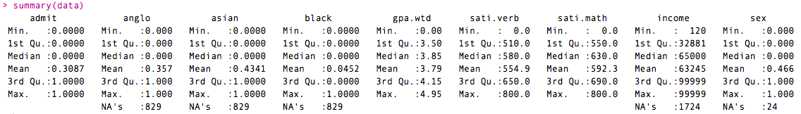
We will now comment on each variable independently. As we can tell from the output above, 2686 of the 8700 applicants were accepted which means admission rate for this university is: 2686/8700 = ~30.89%
When comparing the admission rate for this university (31%) to that of the average 4-Year Private University (62.8%) we learn that it is twice as selective (source).
Because all three of our our predictor variables related to a student’s race capture the same type of information we will analyze them together. We have ethnic data for 6583 or approximately 76% of our test sample, we have 829 observations where there is missing ethnic data.
| Race | Count | Proportion (% of Total) |
|---|---|---|
| Asian | 3417 | 39% |
| African American | 356 | 4% |
| Caucasian | 2810 | 32% |
| NA | 856 | 10% |
| Other | 1261 | 15% |
| Total | 8700 | 100% |
Since the student’s weighted GPA, SAT verbal and SAT Math scores are all numeric data-types, we will create histograms to analyze the distribution of each variable checking for normality and any potential outliers:
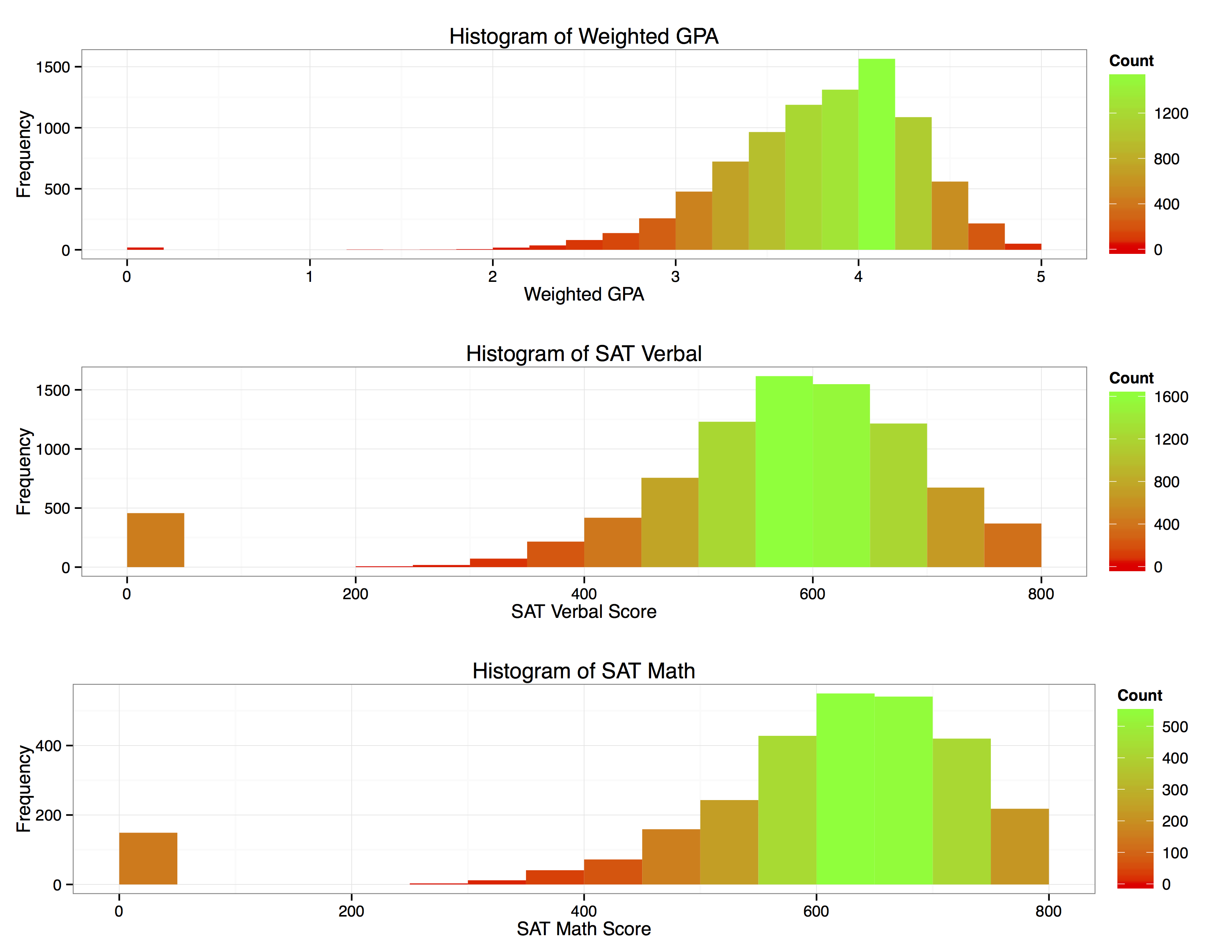
Without performing sophisticated analysis we can tell these data look fairly normally distributed.
However, we must note the large count of ”0s” for SAT scores. Upon investigating it appears that we have missing data for 457 of our sample SAT scores. This should not cause too much concern because it is a relatively small proportion of our total sample. Furthermore, we should not remove the data because we can’t tell if it is missing randomly or if there was systematic recording error present. We will keep these missing values in mind when we move on to model building.
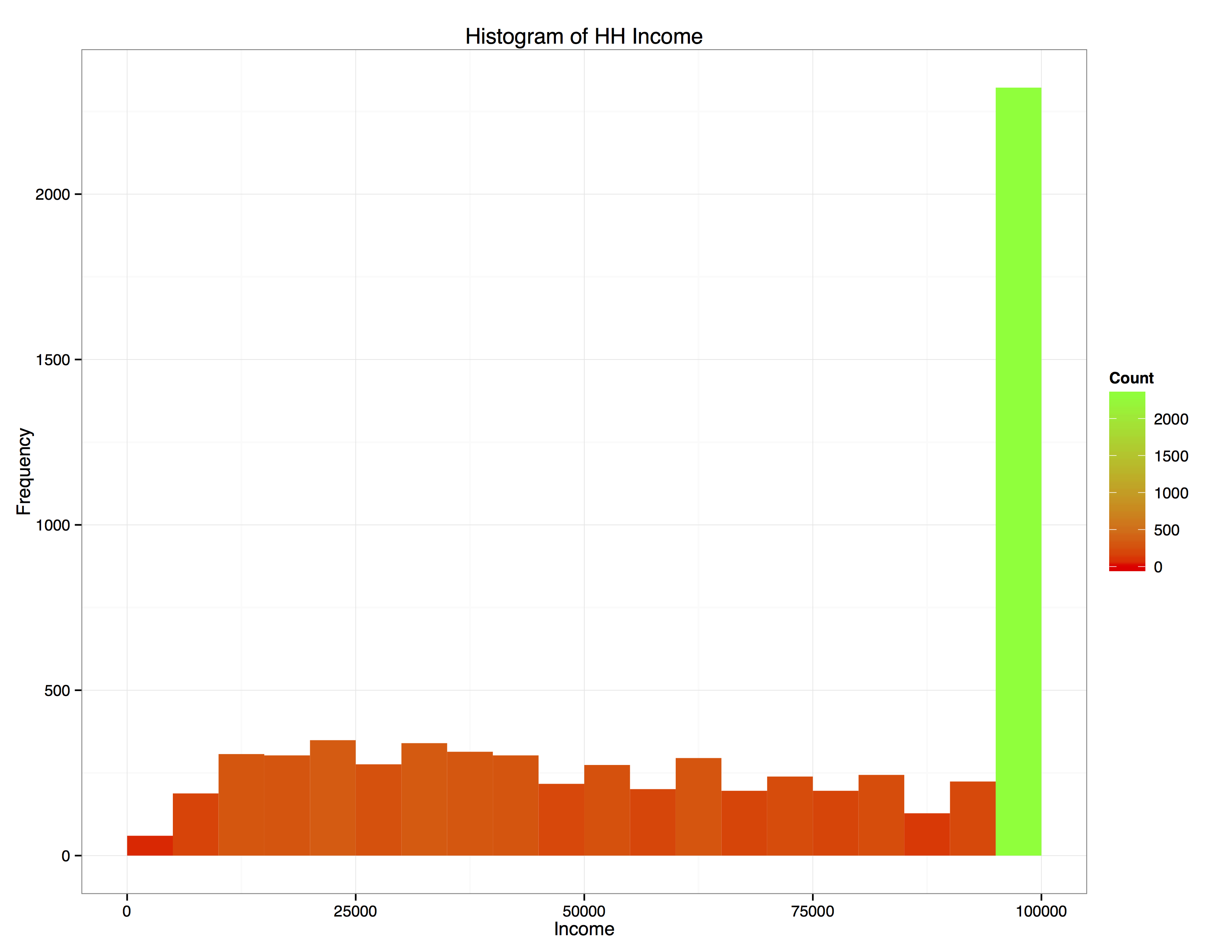
The final variable we will examine is house hold income. It is important to note that all house holds have been capped at an income of $100,000, meaning that all income levels above this cut-off point will be labeled as ”$100,000”. This has a strong effect which becomes evident when we create a histogram of for this variable.
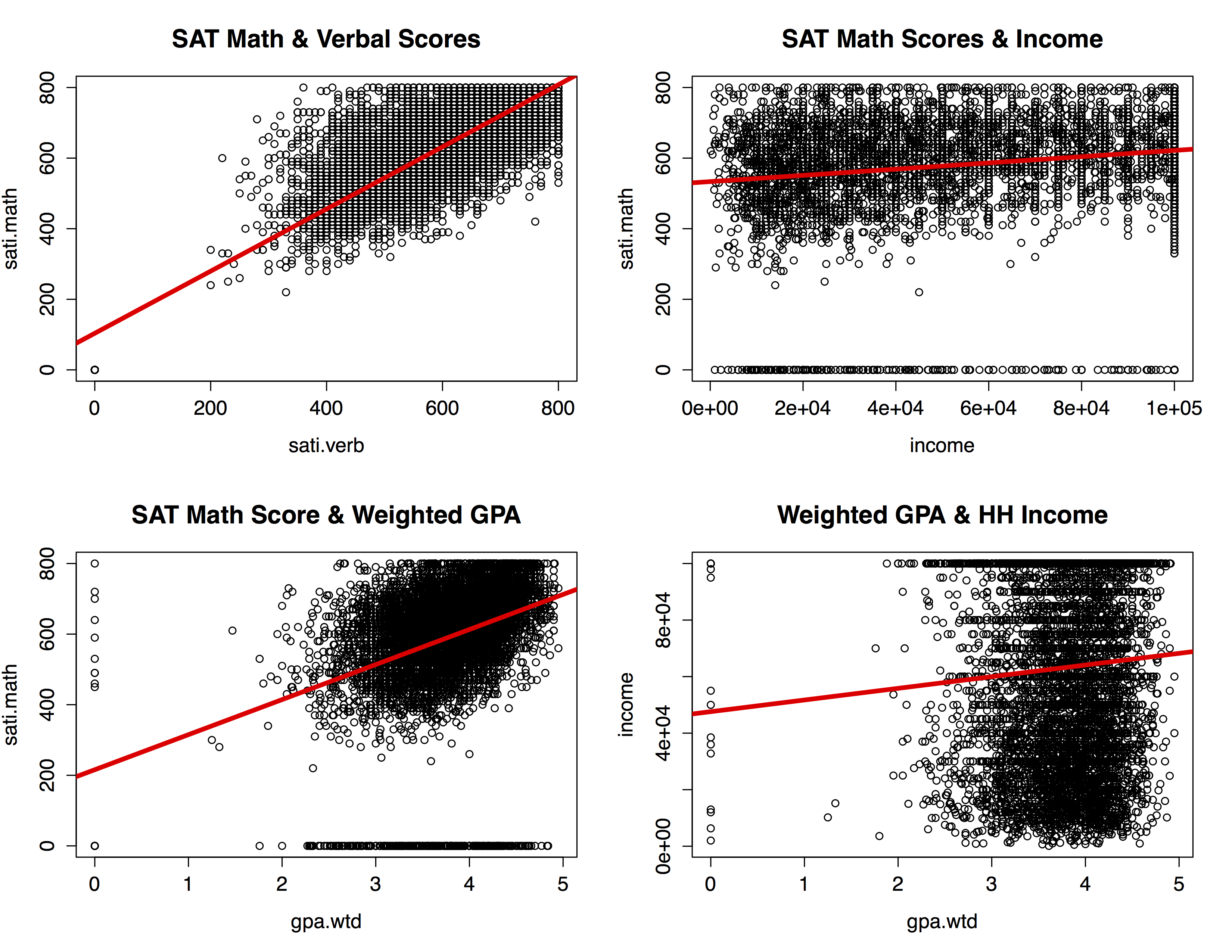
## 3. Multivariate Analysis
We will limit the exploration of multivariate graphs and statistical relationships to numerical data, or specifically: SAT Math and SAT verbal scores, weighted GPA and household income. However, since Math SAT scores and Verbal SAT scores are strongly correlated (R-squared =.736), and thus explain similiar variance within the dataset we will only consider Math scores. Below are summary plots to visualize the relationships between our numerical variables.
## 4. Random Forests Background
4.1 Technicalities
R's CART (Classification And Regression Trees) package which we will use to call the RandomForest function uses the following equation to define a splitting decision:
ΔI(s,A) = I(A) - p(A_L)I(A_L) - p(A_R)I(A_R)
Where I(A) is the value of "impurity" in a parent node, p(A_L) is the likelihood of a given case falling to the left of the parent node and I(A_L) is the impurity of the daughter node resulting from the split, while P(A_R) and I(A_R) capture similar information but for the right daughter node.
Given the above formula the CART algorithm selects a predictor which maximizes ΔI(s,A). By doing so the algorithm is creating terminal nodes which look as homogeneous as possible within the node but as heterogeneous as possible when compared to other terminal nodes. By now it should become clear that Random Forests are simply a large number of decision trees, each node of which is subject to the above optimization (CART Docs).
In reality, the formula for creating a splitting decision is the same for CART as RandomForest, the key difference is that RandomForest creates numerous decision trees sacrificing interpretability for increased predictive power.
5. Model Building With Random Forests
After performing our variable exploration, univariate and bivarate analysis I feel comfortable moving on to building a Random Forest classifier using our data set. Without any model tuning, the algorithm provides the following confusion matrix:
| State | Predicted: Not Admitted | Predicted: Admitted | Model Error |
|---|---|---|---|
| Not Admitted ("0") | 4240 | 308 | 6.7% |
| Admitted ("1") | 716 | 1240 | 36.6% |
| Use Error | 14.5% | 19.9% | Overall Error = 15.7% |
We have created a collection or ”forest” featuring 500 decision trees. In this scenario we have not tuned our parameters and we will accept the default values for priors, this will serve as our baseline model which we can improve upon by tuning priors. The Out of Bag estimate for error rate provided is 15.7%. We also note that our model is under predicting the number of students which should be classified as being admitted (our model predicts 23.8% of students will be admitted but we know from our univariate analysis in section 2.2 that the admit rate should be closer to 31%).
5.1 Calling Random Forests
#-----MODEL BUILDING: RANDOM FORESTS CALL-----
library(randomForest)
# random forests
rf1<-randomForest(admit~.,
              data=data,importance=T, na.action=na.fail, ntree=500)
rf1
5.2 Model Tuning
To correct for the algorithm under predicting the total number of students admitted we introduce priors and assign a cost ratio of 3 to 1. What this means is that we are giving the algorithm ”slack” while predicting whether a student is admitted and tightening our threshold for predicting whether someone is not admitted. After this modification we would expect a false positive rate 3 times greater than a false negative rate.
The reason
for selecting this ratio is because it seems more costly to fail to predict when
someone is admitted compared to the scenario in which a student is classified
as being admitted but was actually not.After running our entire data set through the randomForest() algorithm and setting our cost ration equal to 3 to 1, we arrive at the confusion matrix below:
| State | Predicted: Not Admitted | Predicted: Admitted | Model Error |
|---|---|---|---|
| Not Admitted ("0") | 3536 | 1012 | 22.2% |
| Admitted ("1") | 294 | 1662 | 15% |
| Use Error | 7.7% | 37.9% | Overall Error = 20% |
Notice how the forecasted total number of students admitted went up, increasing the use error but decreasing the model error.
5.3 Model Evaluation
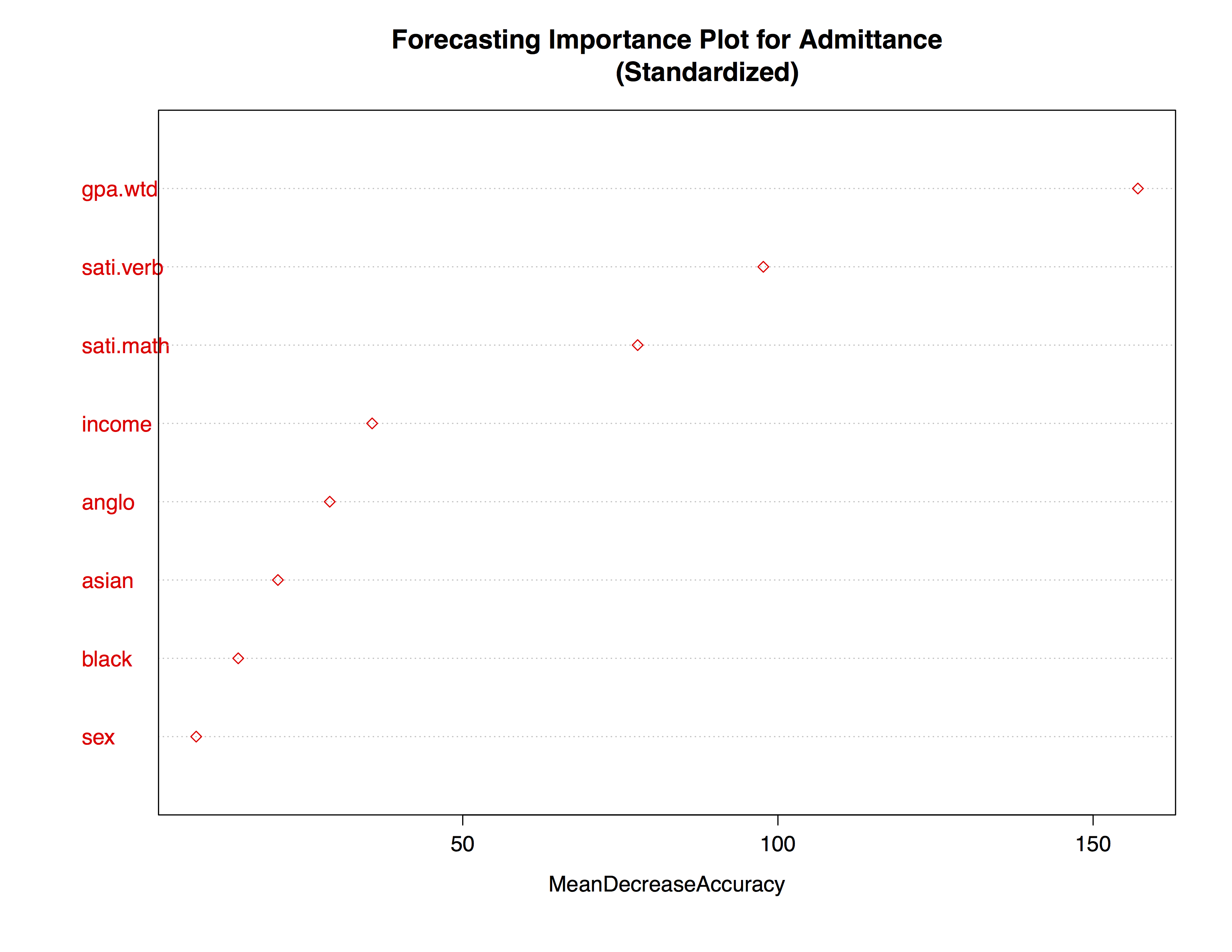
As we see from the plot below the most important variables for predicting whether a student is admitted to this university are those related to academic achievement. For example, Weighted GPA, SAT Math and SAT Verbal Scores explain the most variance within the dataset for our model. While factors like income and race contributed to the accuracy, their effect was less pronounced in our model.
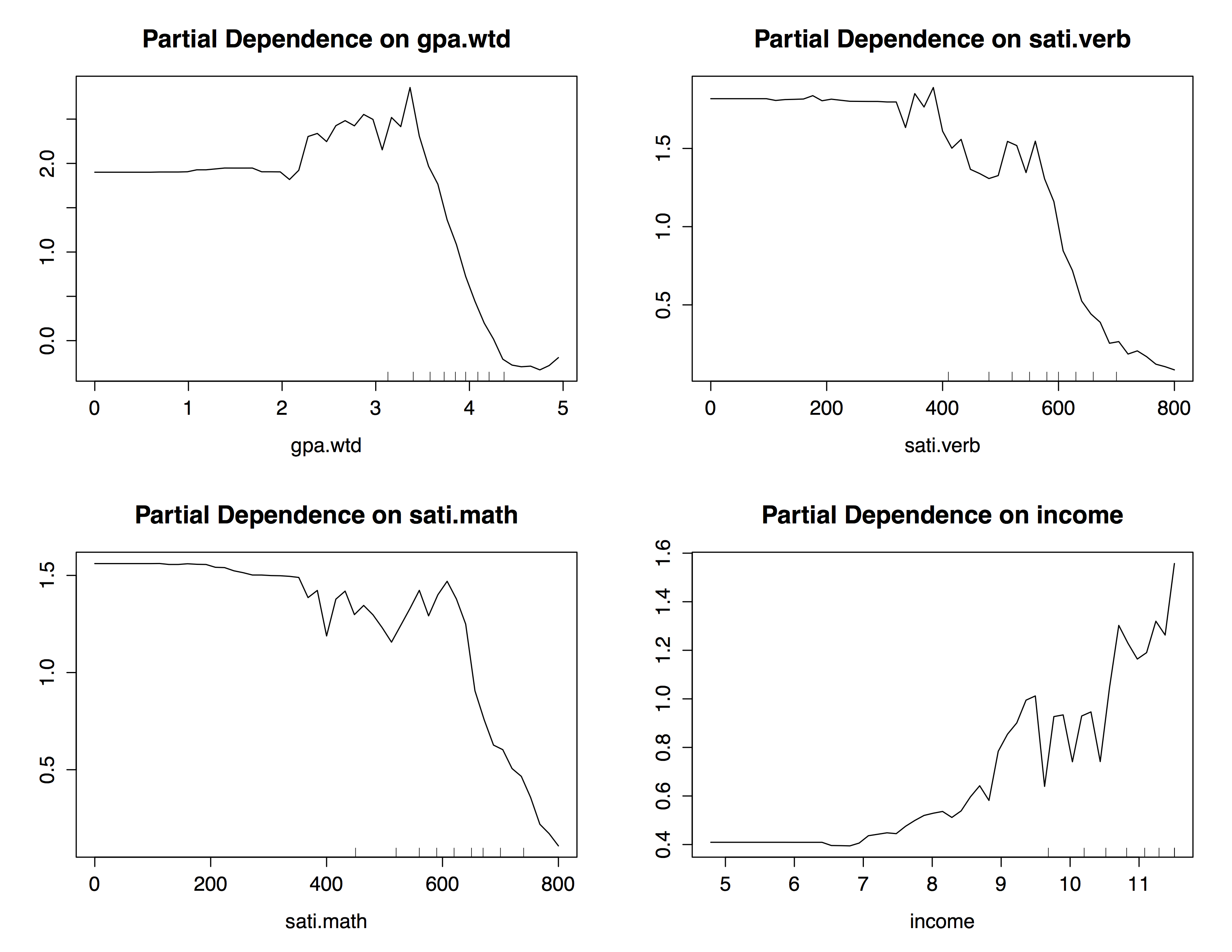
We created partial dependency plots for each of our quantitative variables. The plots for weighted GPA begins to increase at 2.0 and peak around 3.5 meaning that values of weighted GPA between 3 and 3.5 tend to predict ”Admitted = True” strongly. For both SAT verbal and SAT Math scores we see a similar trend. The odds of being admitted increase as levels of income reach above $90,000, see the partial dependency plots below for more details:
5.4 Conclusion
Through this analysis we have gained a deeper understanding into the data behind college admissions. By analyzing the variables available to us we were able to determine that variables related to scholastic performance are much better for predicting the admittance rate of an individual student when compared with socioeconomic and racial factors. We tuned our model to a 3 to 1 cost ratio for false positives and false negatives, meaning we penalized the model by a factor of 3 to 1 when predicting whether a student was accepted. Initially the baseline model produced too many false negatives which was something I had not anticipated. For future analysis I would like to have a larger dataset which includes more than 1 university.