Initial & Exploratory Analysis Method
Phase 1 Initial Analysis
Overview of Initial Data Analysis (IDA)
0.1 What is initial data analysis?
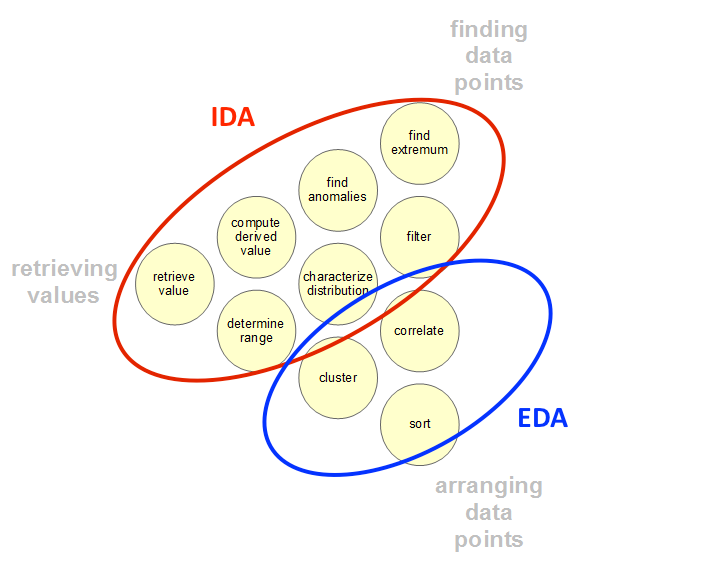
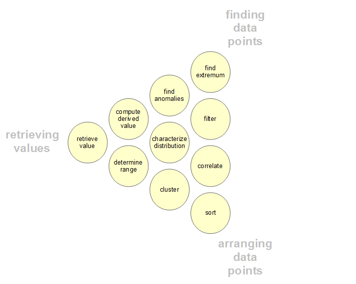
The most important distinction between the initial data analysis phase (IDA) and the main analysis phase (EDA), is that during IDA phase the analyst refrains from any type of activities which directly answer the original research question. Typically the processes in the initial data analysis phase consist of: data quality checks, outlier detection (and treatment), assumption tests and any necessary transformations or imputations for non-normal or missing data. (Source)
0.2 In summary IDA seeks to accomplish the following:
- Uncover underlying structure of the dataset.
- Detect outliers and anomalies.
- Test any necessary underlying assumptions.
- Treatment of problems (typically through transformations or imputations). jerb
1. Understand Underlying Data Structure
1.1 Check the Quality of the Data (Important this happens first)
- Descriptive Summary Statistics (numerically)
- mean
- median
- standard deviation
- size of the data set (number of features & observations)
1.2 Check the Quality of Data Collection Method
- How was the data collected? Do we have any reason to believe the collection process could lead to systematic errors within the data?
2. Detect Outliers and Anomalies
2.1 Check for outliers within the dataset
- Numerically: using range, max-min functions or standard deviation (Rule of thumb: > 2 Standard deviations = potential outlier).
- Visually: histograms.
2.2 Check the normality of the dataset
- This can be accomplished by plotting a frequency distribution (histogram) for each feature (given a small number of features) and identify any skewness present. Here the analyst should also make note of any missing or miscoded data and decide how to handle it (typically through dropping, or transforming).
3. Test Underlying Assumptions
The assumptions the analyst must make will vary based on the model or type of analysis employed. In this example we use the assumptions for linear regression.
3. 1 Assumptions for linear regression:
- Check for no multicollinearity (collinearity)
- Ensure Homoscedasticity
- Linear Relationship
- Normally distributed
- No auto-correlation
4. Treat Potential Problems
At this step the analyst decides to impute missing data, or transform non-normal variables. Transforming variables is a key tool for analysts because it enables her to manipulate the shape of the distribution or nature of the relationship while preserving the information captured by the variable because at any time during the analysis the analyst can reverse the transformation and get the original value of the variable.
4.1 Transformations
| Scenario | Action |
|---|---|
| The variables's distribution differs moderately from the original. | Perform a square root transformation by squaring the observations (x^2). |
| The data's distribution differs significantly from the original. | Perform a log transformation by taking the natural logarithm of the observations (log(x)). |
| The data's distribution differs severe from the original. | Perform an inverse transformation by taking the inverse of a variable (1/x). Another variant would be to take the negative inverse (-1/x) |
| The data's distribution differs severely and none of the above actions worked. | Perform an ordinal transformation by changing the variable's type. |
4.2 Treatment of Problems
After performing necessary transformations, it's vital that the analyst decides how to deal with potential problems and implement any necessary changes within the data before moving onto the next phase.
| Scenario | Action |
|---|---|
| A variable is not normally distributed. | Transform using a technique in table 4.1. |
| The dataset is missing data. | The analyst should either neglect or impute (imputation techniques in R). |
| Significant outliers present. | The analyst should either drop outliers or (depending on the weight they carry) transform the variable. |
| Small sample dataset. | Here, the analyst should consider using bootstrapping, or resampling with replacement, to project the structure of the dataset onto a larger number of observations. |
| NANs & Infs present. | Sometimes datasets will contain NANs or Infs (likely caused by contaminated observations or division by zero) here the analyst must decide to drop the specific observations, or the variable entirely. |
| Incorrect variable types. | This problem is often encountered when dealing with time and monetary variables. Here the analyst should decide to change the variables data type or drop it from the analysis. |
Phase 2: Exploratory Data Analysis (EDA)
Overview of Exploratory Data Analysis (EDA)
5.1 What is exploratory data analysis?
Exploratory data analysis techniques are designed to for open-minded exploration and not guided by a research question. EDA should not be thought of as an exhaustive set of steps to be strictly followed but rather a mindset or philosophy the analyst brings with her to guide her exploration.
The analyst uses EDA techniques to “tease out” the underlying structure of the data and manipulate it in ways that will reveal otherwise hidden patterns, relationships and features. EDA techniques are primarily graphical because humans have innate pattern recognition abilities which we utilize to synthesize complex conclusions from visual cues.
The goal of EDA is to accomplish the following:
- Maximize insight into a data set.
- Understand and rank variables by importance.
- Determine the optimal trade-offs between parsimonious and accurate models.
- Determine optimal factor settings (such as tuning priors or making manual adjustments to statistical algorithms).
5.2 EDA Steps:
- Plot raw data.
- Plot simple statistics.
- Position the plots in a manner than maximizes the number of inferences a viewer can make while minimizing the both the time it takes and the "Data-ink ratio" used to arrive at these insights.
- (Optional) Leverage the insights from the graphical and statistical analysis to inform model building activities such as feature selection, transformation, and tuning.
Some of these steps may seem redundant but it's important to remember that any transformations or significant adjustments to the dataset should have been carried out in the IDA phase. In the EDA phase we must ensure these adjustments had the intended effect and do not contaminate or misrepresent the dataset.
(Source: Engineering Statistics Handbook)
6. Plotting Raw Data
6.1 Bivaraite Analysis
- Re-examine the frequency distribution of each variable (for a small number of variables) and ensure they meet expectations. If transformation or imputation has been performed on the variable, note the effect.
- Histograms
6.2 Multivariate Analysis
- Begin to examine the nature of the relationships between variables within the dataset. Here the analyst should note any strong relationships (linear or otherwise) or potentially confounding variables which will inform variable selection if model building is the intended goal.
- Scatter Plots
- Pairs Plots (Python:
seaborn.pairs(), R:pairs())
7. Plotting Simple Statistics
7.1 Simple Summary Statistics
-
Similiar to step 1.1, except we must re-examine the summary statistics for transformed or imputed variables, except this time with an emphasis on analyzing the information visually.
- Mean
- Median
- Standard deviation
- Box plots (or quantile plots)
- Size of the data set (number of features & observations)
- Especially if observations or features were dropped or bootstrapped in phase 4.2.
-
Helpful Functions
8. Position & Present
8.1 Presenting the findings
At this point in the exploration the analyst should have: 1. An understanding of the underlying data structure (visually & numerically). (1.1, 1.2, 6.1, 7.1) 2. Insight into the relationships between variables. (6.2) 3. The impact of transformations, imputations or any other significant changes to the original dataset. (4.1, 4.2)
The analyst should now feel comfortable positioning their plots and summary statistics in a manner than maximizes the number of inferences a viewer can make while minimizing the both the time it takes and the amount of ink used to arrive at these insights . This could be in the form of a dash board, a single visualization, multiple visualizations or any other acceptable medium of presentation with the goal presenting the data in a manner that engages the viewer and challenges them to ponder its impact and implications (Source: Introduction to Survey Design).
9. Model Building
Model building is typically the final stage of any analysis. It comes last because the analyst should have a deep understanding of the dataset and how the variables relate to one another. Posessing this information will simplify the following.
9.1 Model Selection
- What is the goal of the model?
- How big is the data set? (observations)
- How many features are contained in the dataset? (variables)
- Does the data lend itself to supervised or unsupervised machine learning methods?
9.2 Model Fitting
- Break the dataset into training and testing sets (Rule of thumb: 80/20 split).
- Feature Selection & Ranking
- Selecting your algorithm there are many.
9.3 Model Validation
- Fit the model you selected in 9.1 to your training set and run the testing set through the model to determine its error rate.
- This rate will differ between modeling techniques.
- Perform model tuning by adjusting for things like type I and type II error, re-fitting the model after each adjustment.
9.4 EDA Conclusion
At the end of the EDA process, the analyst should have the following: - Treatment for outliers and abnormal data. - A ranked list of a dataset’s features and how they contribute to the model. - Conclusions or insights arrived at as a result of the exploratory analysis. - A statistically sound and parsimonious model.
Guding EDA Questions
- What is a typical value for a given feature within a dataset?
- How is the data distributed?
- Does a given factor have a significant effect on an outcome?
- What are the most important factors for predicting a given response variable?
- What is the best model for forecasting unknown values of a response variable?
- What is signal vs noise in time series data?
- Does the dataset have outliers?